Spin and the Periodic Table

We have navigated through the three spatial dimensions of the atom—the size ($n$), the shape ($\ell$), and the orientation ($m_{\ell }$) of electron orbitals. However, our model is not yet complete. Even with these three quantum numbers, experimental results (like the Stern-Gerlach experiment) showed that electrons have one more property that defines their behavior.

To finish the puzzle, we must add the fourth and final quantum number: Spin.

6.1 The Fourth Dimension: Spin ($m_s$)

In 1922, Otto Stern and Walther Gerlach discovered that a beam of silver atoms, when passed through a non-uniform magnetic field, split into exactly two distinct paths. This "splitting" couldn't be explained by orbital motion alone. It suggested that electrons possess an intrinsic magnetic moment, as if they were tiny spinning charges. Silver is an apt choice here: a silver atom's closed inner shells carry no net angular momentum, so its entire magnetic response comes from a single unpaired outer electron — and because that electron occupies an $s$ orbital ($\ell =0$), it has no orbital motion to contribute, leaving the two beams to map directly onto its two spin states.

The Spin Quantum Number, $m_s$

Unlike the spatial quantum numbers, which arise from the geometry of 3D space, Spin is an intrinsic property of the electron itself.

• Allowed Values: $m_s=+1/2$ (Spin-Up) or $m_s=-1/2$ (Spin-Down).
• Physical Meaning: While we often visualize the electron as a tiny planet spinning on its axis, this is just an analogy. In reality, spin is a fundamental form of angular momentum that has no classical counterpart.

6.2 The Four Quantum Numbers

Every electron in an atom is uniquely described by four quantum numbers. No two electrons can share all four — this is the Pauli Exclusion Principle.

• $n$ (Principal): Energy shell / distance from nucleus. Allowed values: 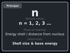$1,2,3,\dots$

  

• $\ell$ (Azimuthal): Subshell shape. Allowed values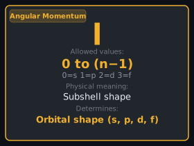: $0$ to $n-1$ ($0=s$, $1=p$, $2=d$, $3=f$)

  

• $m_{\ell }$ (Magnetic): Orbital orientation in space. Allowed values: $-\ell$ to $+\ell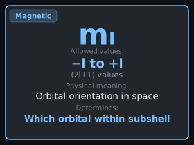$ ($2\ell +1$ values)

  

• $m_s$ (Spin): Intrinsic electron spin. Only two values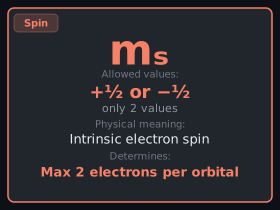: $+1/2$ or $-1/2$

  

Total states in shell $n$

Each principal shell $n$ contains $n$ subshells ($\ell =0,1,\dots ,n-1$). Each subshell $\ell$ provides $2\ell +1$ distinct orientations ($m_{\ell }$ values), and each orientation holds 2 electrons (one spin-up, one spin-down). Summing over all subshells:

$$\text{Total electrons in shell }n=2\sum _{\ell =0}^{n-1}(2\ell +1)=2n^2$$

$n$	Shell	Subshells	Electrons per subshell	Total $2n^2$
1	K	$1s$	2	2
2	L	$2s,2p$	2 + 6	8
3	M	$3s,3p,3d$	2 + 6 + 10	18
4	N	$4s,4p,4d,4f$	2 + 6 + 10 + 14	32
5	O	$5s,5p,5d,5f,(5g)$	2 + 6 + 10 + 14 + 18	50
6	P	$6s,6p,6d,\dots$	2 + 6 + 10 + 14 + 18 + 22	72
7	Q	$7s,7p,\dots$	2 + 6 + 10 + 14 + 18 + 22 + 26	98

Subshell capacity: $s=2,p=6,d=10,f=14$ — each equals $2(2\ell +1)$, i.e. 2 electrons per orientation.

6.3 The Pauli Exclusion Principle

With four quantum numbers in hand, we can now state the most important rule in chemistry, formulated by Austrian physicist Wolfgang Pauli in 1925:

The Rule:

No two electrons in the same atom can have the exact same set of four quantum numbers:
($n,\ell ,m_{\ell },m_s$)

The Consequence: Orbital Capacity

This principle limits how many electrons can "live" in a single orbital.

1. An orbital is defined by a unique set of ($n,\ell ,m_{\ell }$).
2. Inside that orbital, there are only two possible values for $m_s$ ($+1/2$ or $-1/2$).
3. Therefore, each orbital can hold a maximum of 2 electrons, and they must have opposite spins.

This simple rule is why matter occupies space. Without it, all electrons would collapse into the lowest energy state ($1s$), and chemistry as we know it would not exist.

6.4 The Building Blocks: Aufbau and Hund

To build an atom, we "fill" the orbitals with electrons starting from the lowest energy state and working our way up. This process is governed by two key rules:

1. The Aufbau Principle (Building Up)

The Aufbau Principle (German for "building up") states that electrons fill the lowest available energy subshell first. In multi-electron atoms, subshells of the same principal quantum number $n$ are no longer degenerate: penetration and shielding split them so that $E_{ns}<E_{np}<E_{nd}<E_{nf}$, and this splitting can even make a higher-$n$ subshell (like $4s$) lower in energy than a lower-$n$ one (like $3d$). The diagonal rule (Madelung rule) gives a practical mnemonic: fill in order of increasing $n+\ell$, and for equal $n+\ell$, in order of increasing $n$.

Electrons fill subshells in order of increasing energy:

$$\begin{array}{rl}& 1s\to 2s\to 2p\to 3s\to 3p\to 4s\to 3d\to 4p\to 5s\to 4d\\ & \to 5p\to 6s\to 4f\to 5d\to 6p\to 7s\to 5f\to 6d\to 7p\end{array}$$

Mnemonic: The $(n+\ell )$ Rule To quickly find which subshell has lower energy, calculate the sum of $n$ and $\ell$.

1. The subshell with the lower $(n+\ell )$ value fills first.
2. If the values are equal, the subshell with the lower $n$ fills first.

Example: 4s ($4+0=4$) vs. 3d ($3+2=5$). Since $4<5$, 4s fills first. Example: 3d ($3+2=5$) vs. 4p ($4+1=5$). Since the sums are equal, 3d fills first ($n=3$ is lower than $n=4$).

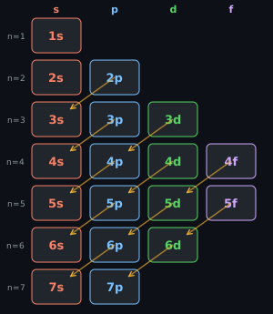
Subshell grid — each $(n,\ell )$ cell is a subshell; diagonal arrows trace the Aufbau filling sequence.

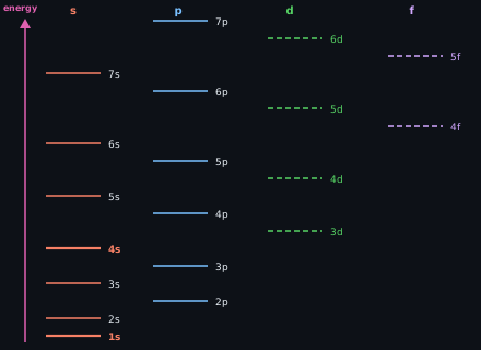
Energy levels (filling order ↑) — subshells ranked from lowest energy (1s, bottom) to highest (7p, top) in a multi-electron atom.

The energy diagram reveals the key insight: 4s fills before 3d because 4s has lower energy for $Z<21$, even though $n=4>n=3$. This is a direct consequence of the penetration and shielding effects described in Chapter 5.

A key concept in understanding the Aufbau filling order is the crossing of energy levels in multi-electron atoms. While Hydrogen has degenerate $n$ levels (all $n=3$ subshells have the same energy), multi-electron atoms show a different ordering due to penetration and shielding. As atomic number $Z$ increases, subshell energies shift: $4s$ dips below $3d$ for light atoms, then $3d$ drops back below $4s$ for heavier ones. This resembles — but is not — hysteresis: it is a smooth, one-way energy inversion as $Z$ increases (hysteresis would require the system to return via a different path; here the crossing is permanent and monotonic).

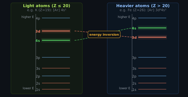
Energy level inversion — the relative ordering of 4s and 3d flips between light and heavier atoms; the dashed curves trace which orbital is which across the two regimes.

The diagram shows:

• In light atoms ($Z\le 20$): $4s$ sits below $3d$ in energy — $4s$ fills first (e.g. K: [Ar] 4s¹)
• In heavier atoms ($Z>20$): once $3d$ starts filling, it drops below $4s$ — the levels permanently invert (e.g. Fe: [Ar] 3d⁶4s²)
• Ionization paradox: Fe is [Ar]3d⁶4s² in the ground state, but when ionized to Fe²⁺ it loses the $4s$ electrons first, giving [Ar]3d⁶ (not [Ar]3d⁴4s²). Once $3d$ starts filling it drops below $4s$, making $4s$ the highest-energy electrons — they leave first upon ionization.

2. Hund's Rule (The Bus Passenger Rule)

When filling a subshell with multiple orbitals (like the three $2p$ orbitals), electrons prefer to occupy empty orbitals singly with parallel spins before they start pairing up.

Analogy: Like passengers on a bus, electrons take an empty seat before sitting next to someone else. This minimizes electron-electron repulsion and makes the atom more stable.

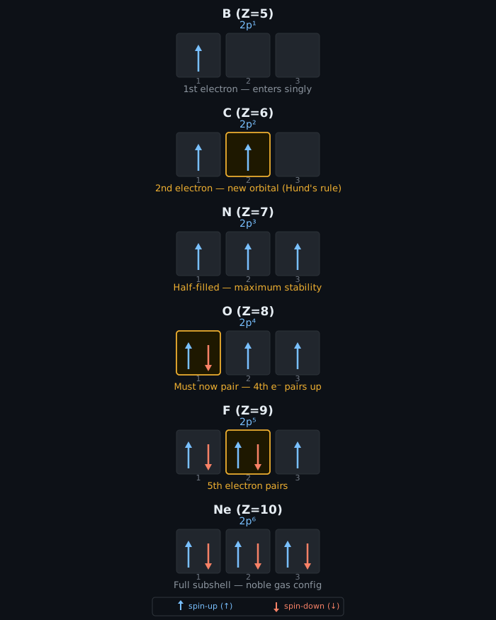
The diagram illustrates how electrons fill the three $2p$ orbitals: each orbital receives one spin-up electron first (B → N), then electrons pair up as the subshell fills (O → Ne).

3. Exceptions to the Rule

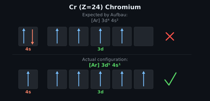
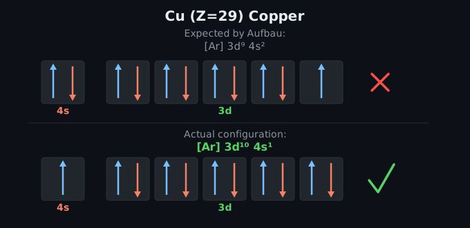
Nature occasionally breaks the Aufbau sequence to achieve even greater stability. The most famous examples are Chromium (Cr) and Copper (Cu).

• Half-filled Stability: Chromium ($Z=24$) is expected to be $[Ar]3d^{4}4s^2$, but it is actually $[Ar]3d^{5}4s^1$. Having five electrons in the $d$-subshell (one in each orbital) provides extra "exchange energy" stability.

• Fully-filled Stability: Copper ($Z=29$) is expected to be $[Ar]3d^{9}4s^2$, but it is actually $[Ar]3d^{10}4s^1$. A completely full $d$-subshell is more symmetric and stable.

Beyond Chromium and Copper, the $d$-block holds ten well-known Aufbau exceptions — elements whose measured ground-state configuration differs from the naive Madelung prediction. In each, the $d$ and $s$ subshell energies lie close enough that a half-filled or fully-filled $d$-subshell outweighs the cost of leaving the outer $s$-orbital singly occupied:

Element	$Z$	Aufbau prediction	Actual configuration	Gain
Cr	24	$[Ar]3d^{4}4s^2$	$[Ar]3d^{5}4s^1$	half-filled $3d$
Cu	29	$[Ar]3d^{9}4s^2$	$[Ar]3d^{10}4s^1$	fully-filled $3d$
Nb	41	$[Kr]4d^{3}5s^2$	$[Kr]4d^{4}5s^1$	exchange energy
Mo	42	$[Kr]4d^{4}5s^2$	$[Kr]4d^{5}5s^1$	half-filled $4d$
Ru	44	$[Kr]4d^{6}5s^2$	$[Kr]4d^{7}5s^1$	exchange energy
Rh	45	$[Kr]4d^{7}5s^2$	$[Kr]4d^{8}5s^1$	exchange energy
Pd	46	$[Kr]4d^{8}5s^2$	$[Kr]4d^{10}$	fully-filled $4d$, no $5s$
Ag	47	$[Kr]4d^{9}5s^2$	$[Kr]4d^{10}5s^1$	fully-filled $4d$
Pt	78	$[Xe]4f^{14}5d^{8}6s^2$	$[Xe]4f^{14}5d^{9}6s^1$	exchange energy
Au	79	$[Xe]4f^{14}5d^{9}6s^2$	$[Xe]4f^{14}5d^{10}6s^1$	fully-filled $5d$

Palladium ($Z=46$) is the most extreme case: it abandons the outer $5s$ electrons entirely in favor of a completely filled $4d^{10}$ subshell — the only element with no electrons in its outermost $s$ orbital at ground state.

The $d$-block is not the whole story. Many lanthanides and actinides are irregular too — there the $4f$, $5d$ and $6s$ levels (or $5f$, $6d$ and $7s$ in the actinides) lie so close together that anomalous configurations are common. Those follow a more tangled pattern and are left out of the table above for clarity.

6.5 Paramagnetism and Diamagnetism

A direct consequence of Hund's rule is that many atoms have unpaired electrons — electrons occupying an orbital singly, with no partner of opposite spin. This determines how an atom responds to an external magnetic field:

• Paramagnetic — one or more unpaired electrons. Each acts as a tiny bar magnet (spin magnetic moment). In a field the moments align, and the atom is weakly attracted.
• Diamagnetic — all electrons paired. No net spin moment; the atom is very weakly repelled.

The diagram below shows the orbital filling for the first ten elements. Each box is one orbital; a single arrow (↑) is one electron, a paired arrow pair (↑↓) is two.

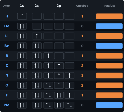
Hund's rule is visible in the 2p filling: B through N take one electron each (maximizing unpaired spins), then O through F start pairing as the subshell fills. Nitrogen (3 unpaired) is the most paramagnetic in the row. Helium, Beryllium, and Neon have all electrons paired — they are diamagnetic.

Quick rule

Count unpaired electrons in the orbital box diagram.
0 → diamagnetic
1+ → paramagnetic

6.6 Electron Shell Diagrams

The Bohr shell model represents electrons as colored dots on concentric rings around the nucleus. Each ring is a principal shell ($n=1,2,\dots$). Within each shell, electrons occupy subshells by type: s (orange), p (blue), d (green), f (purple). Filled dots show electrons present; empty circles mark available but unoccupied slots.

Shell capacity

Each principal shell $n$ holds at most $2n^2$ electrons, distributed across its subshells:

Shell	Subshells	Capacity
$n=1$	$1s$	$2$
$n=2$	$2s,2p$	$8$
$n=3$	$3s,3p,3d$	$18$
$n=4$	$4s,4p,4d,4f$	$32$

Electrons fill subshells in order of increasing $n+\ell$ (Madelung rule), and within the same $n+\ell$ in order of increasing $n$ — the diagonal rule from section 6.4.1.

Explore any element

Pick any of the 118 elements below to see two complementary views of its ground-state configuration, both built on the fly from the actual electron configuration:

• Bohr shell model — electrons as colored dots on concentric shell rings, with a green nucleus labeled by its proton count. Toggle show all subshells to reveal every subshell of each occupied shell, including the empty ones, drawn as faint slots in the subshell color.
• Subshell energy levels — occupied subshells placed at their actual DFT orbital energies (NIST LDA data), lowest energy at the bottom. Each subshell's orbitals appear as boxes filled with ↑/↓ spin arrows following Hund's rule; the box-group width is proportional to subshell capacity ($s$ narrowest, $f$ widest). Toggle show empty subshells to display unoccupied subshells above the energy scale in schematic Madelung order.

For the 10 Aufbau exceptions from section 6.4.3, the energy diagram marks the subshells whose actual occupancy differs from the naive $(n+\ell )$ prediction with a gold ★ — for example chromium's $3d^{5}4s^1$ instead of the predicted $3d^{4}4s^2$.

show all subshells show empty subshells energy ladder only

Energy scale. The upper section of the energy ladder is a linear scale from 0 to −30 eV, so spatial gaps between subshells reflect real energy differences — a 5 eV separation looks twice as wide as a 2.5 eV one. Orbital energies come from NIST density-functional theory (LDA) calculations for the neutral atom ground state. Deep core levels (below −30 eV) are compressed into the lower band, shown only for completeness; they are chemically inert and never reorder relative to each other. Unoccupied subshells, when shown, appear above the scale in schematic Madelung order without energy claims.

Energy-level crossings. Subshell energies shift as $Z$ increases, and several pairs cross — the same physics that creates the 4s/3d inversion shown in section 6.4.1 repeats across the periodic table:

Crossing	Occurs at	Effect
4s / 3d	Sc–Ti (Z = 21–22)	4s fills first in K and Ca; 3d drops below 4s as the transition series opens at Sc–Ti. Cr (Z = 24) briefly reverses due to its half-filled-3d anomaly.
5s / 4d	Mo (Z = 42)	Exact analogue in the 4d series: 5s fills first in Rb and Sr, then 4d sinks below 5s. Nb (Z = 41) shows a similar transient reversal.
6s / 5d	La (Z = 57)	5d drops below 6s at the very start of the lanthanide period, simultaneously with 4f beginning to compete — three subshells near-degenerate.
6s / 4f	Ce–Sm region	As the lanthanides fill, 4f deepens rapidly below 6s while 5d remains close; this three-way near-degeneracy is why lanthanide configurations are the most complex in the table.
7s / 5f, 6d	Th–Pa (Z ≥ 90)	The same pattern recurs in the actinides, compounded by strong relativistic effects at high Z.

To see a crossing in action, step through the element selector: Ca → Sc → Ti watches the 3d level sink from above 4s to below it; Ba → La shows the 5d/6s inversion.

6.7 Valence Fill — All 118 Elements

With the Aufbau rules established and representative shell diagrams in hand, the table below shows the complete picture: how every element from hydrogen to oganesson fills its valence subshells.

Each row is one element. The s / p / d / f columns show a fill bar and fraction (electrons present / subshell capacity: s = 2, p = 6, d = 10, f = 14), drawn from the actual ground-state configuration. The 10 Aufbau exceptions from section 6.4 are marked ★ with a gold row highlight.

0 / 118

Z	Symbol	Name	s	p	d	f

6.8 The Periodic Table Emerges

The entire structure of the periodic table is a direct "map" of these quantum rules.

The Blocks

The table is divided into four blocks based on which subshell is being filled. The block widths — s: 2, f: 14, d: 10, p: 6 columns — are exactly the subshell capacities $2(2\ell +1)$.

True ordering: 32 columns

In strict quantum order, blocks run s · f · d · p left to right within each period. Every fully-filled period spans exactly 2 + 14 + 10 + 6 = 32 elements — which is why the lanthanides and actinides each hold 14 elements, the transition metals 10, and the main-group p-elements 6. Dashed outlines mark subshells not yet filled in that period.

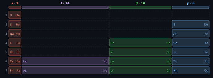
Empty boxes: subshell exists but is not yet reached in the Aufbau order for that period. Colored bars: first and last element of each filled block.

Practical layout: 18 columns

Printing a 32-column table is impractical. The standard solution is to extract the f-block and display it below the main body, collapsing the width to 2 + 10 + 6 = 18 columns. This is the familiar periodic table that everyone recognizes — a layout choice, not a quantum one.

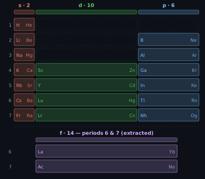
f-block (14 columns) detached to reduce width — it belongs between s and d in periods 6 and 7.

Why the offsets?

You may notice that in Period 4, we fill the $3d$ subshell, and in Period 6, we fill $4f$. As explained in Chapter 5, the $s$ orbitals of a higher shell ($n$) penetrate so well that they actually have lower energy than the $d$ or $f$ orbitals of lower shells. Thus, $4s$ is more stable than $3d$, and $6s$ is more stable than $4f$.

The Magic Numbers

The lengths of the periods come directly from the orbital capacities ($s=2,p=6,d=10,f=14$):

• Period 1: $1s$ (2e) = 2 elements (H, He).
• Period 2: $2s$ (2e) + $2p$ (6e) = 8 elements (Li $\to$ Ne).
• Period 3: $3s$ (2e) + $3p$ (6e) = 8 elements (Na $\to$ Ar).
• Period 4: $4s$ (2e) + $3d$ (10e) + $4p$ (6e) = 18 elements (K $\to$ Kr).
• Period 5: $5s$ (2e) + $4d$ (10e) + $5p$ (6e) = 18 elements (Rb $\to$ Xe).
• Period 6: $6s$ (2e) + $4f$ (14e) + $5d$ (10e) + $6p$ (6e) = 32 elements (Cs $\to$ Rn).
• Period 7: $7s$ (2e) + $5f$ (14e) + $6d$ (10e) + $7p$ (6e) = 32 elements (Fr $\to$ Og).

Who invented these representations? 🤔

Two scientists, a century apart, each gave us one of the two layouts above.

Dmitri Mendeleev (Russian chemist, 1834–1907) published the first widely recognized periodic table in 1869, arranging the 63 elements then known by increasing atomic weight and lining up similar chemical behaviors in columns. He famously left gaps for undiscovered elements — and predicted their properties with remarkable accuracy (gallium, germanium, and scandium were all found later, matching his forecasts). The 18-column table in common use today is the direct descendant of his arrangement; the name Mendeleev's periodic table is still standard in chemistry.

Charles Janet (French engineer and amateur naturalist, 1849–1932) proposed the 32-column layout in 1928. Working outside academic chemistry, he published it privately, which delayed its recognition by decades. His insight was to arrange elements strictly by the Aufbau / Madelung $(n+\ell )$ filling rule, placing blocks in the order s → f → d → p from left to right so that every row corresponds to one complete quantum shell. The result — sometimes called the left-step or Janet periodic table — is the truer quantum map. Its one notable quirk: helium moves to group 2 next to beryllium, because its configuration 1s² is s-block, whereas in Mendeleev's table it sits in group 18 for chemical-behavior reasons.

In short: Mendeleev gave us a tool for chemistry; Janet gave us a tool for quantum mechanics.

6.9 Conclusion: The Quantum Atom

We have traveled from the abstract wave function of Chapter 1 to the concrete structure of the 118 elements. The periodic table is not just a list of ingredients; it is a mathematical consequence of the laws of quantum mechanics.

By solving the Schrödinger equation and applying the rules of Spin and Exclusion, we have revealed the hidden logic of the universe—showing that the complexity of matter emerges from the elegant simplicity of quantum numbers.

---

References:

• Mathematical Annex: Mathematical formulas and 3D visualizations.
• Elements Reference: Complete data for all 118 elements.