The Shapes of Probability (The Angular Solution)

In Chapter 3, we successfully separated the Schrödinger equation into a Radial part ($R$) and an Angular part ($Y$). Now, we dive into the math of the angles.

Solving this equation will reveal why electrons don't just sit in simple spheres, but instead occupy the complex "dumbbells" and "donuts" that define the $p,d,$ and $f$ blocks of the periodic table.

4.1 The Angular Equation

From our separation in Chapter 3, we have the following equation for $Y(\theta ,\varphi )$:

$$\frac{1}{\sin \theta }\frac{\partial }{\partial \theta }(\sin \theta \frac{\partial Y}{\partial \theta })+\frac{1}{{\sin }^2\theta }\frac{{\partial }^{2}Y}{\partial {\varphi }^2}=-\ell (\ell +1)Y$$

Notice that this equation is independent of the nucleus's charge ($Z$) or the particle's mass ($m$). This means the shapes of orbitals are universal—a $p$-orbital in Hydrogen looks exactly like a $p$-orbital in Gold.

4.2 Splitting the Angles Again

To solve for $Y(\theta ,\varphi )$, we apply Separation of Variables one more time. We assume that the angular function is itself a product of two independent functions:

$$Y(\theta ,\varphi )=\mathrm{\Theta }(\theta )\cdot \mathrm{\Phi }(\varphi )$$

Why is this separation valid? 🤔

This works because the $\theta$ and $\varphi$ operators in the Laplacian are "orthogonal." Changing the angle around the equator ($\varphi$) doesn't change the radius or the angle from the pole ($\theta$). Mathematically, the variables are independent parts of the same spherical surface.

By substituting this product into our angular equation and multiplying by ${\sin }^2\theta /(\mathrm{\Theta }\mathrm{\Phi })$, we can pull the $\varphi$ terms to one side:

$$\underset{\text{Depends only on }\theta }{\underbrace{\frac{\sin \theta }{\mathrm{\Theta }}\frac{d}{d\theta }(\sin \theta \frac{d\mathrm{\Theta }}{d\theta })+\ell (\ell +1){\sin }^2\theta }}=\underset{\text{Depends only on }\varphi }{\underbrace{-\frac{1}{\mathrm{\Phi }}\frac{d^2\mathrm{\Phi }}{d{\varphi }^2}}}$$

Just as before, for both sides to stay equal, they must equal a constant. We call this constant $m_{\ell }^2$.

Why the "Squared" Integer? 🤔

Mathematically, a second-order derivative that returns the negative of itself (${\mathrm{\Phi }}^{″}=-C\mathrm{\Phi }$) has sine and cosine solutions. By choosing a squared constant ($m_{\ell }^2$), we ensure the solution is in the form of a harmonic wave. And as we'll see in the next section, the "boundary" of ${360}^{\circ }$ will force $m_{\ell }$ to be a whole integer.

4.3 Solving for $\varphi$: The Magnetic Quantum Number ($m_{\ell }$)

The equation for $\mathrm{\Phi }$ is the simplest differential equation in quantum mechanics:

$$\frac{d^2\mathrm{\Phi }}{d{\varphi }^2}=-m_{\ell }^2\mathrm{\Phi }$$

The solution is a complex exponential:

$$\mathrm{\Phi }(\varphi )=\exp (i{m}_{\ell }\varphi )$$

The Physical Constraint: If you rotate ${360}^{\circ }$ ($2\pi$ radians) around an atom, you must end up exactly where you started. Therefore, $\mathrm{\Phi }(\varphi )$ must equal $\mathrm{\Phi }(\varphi +2\pi )$.

$$\exp (i{m}_{\ell }\varphi )=\exp [i{m}_{\ell }(\varphi +2\pi )]⟹\exp (i2\pi m_{\ell })=1$$

This is only true if $m_{\ell }$ is an integer ($\cdots -2,-1,0,1,2\dots$). This $m_{\ell }$ is our second Quantum Number, the Magnetic Quantum Number, which determines the orbital's orientation in space.

4.4 Solving for $\theta$: The Azimuthal Quantum Number ($\ell$)

The equation for $\mathrm{\Theta }(\theta )$ is much more challenging:

$$\sin \theta \frac{d}{d\theta }(\sin \theta \frac{d\mathrm{\Theta }}{d\theta })+[\ell (\ell +1){\sin }^2\theta -m_{\ell }^2]\mathrm{\Theta }=0$$

This is a famous mathematical equation known as the Associated Legendre Equation. Its solutions are the Associated Legendre Polynomials, $P_{\ell }^{m_{\ell }}(\cos \theta )$:

$$P_{\ell }^{m_{\ell }}(x)=\frac{(-1{)}^{m_{\ell }}}{2^{\ell }\ell !}(1-x^2{)}^{m_{\ell }/2}\frac{d^{\ell +m_{\ell }}}{d{x}^{\ell +m_{\ell }}}(x^2-1{)}^{\ell }$$

For a detailed derivation and historical context of these polynomials, see the Mathematical Annex.

The Physical Constraint: For these polynomials to remain finite (not blow up to infinity at the poles), the constant $\ell$ must be an integer, and it must satisfy:

$$\ell \ge |m_{\ell }|$$

This gives us our third Quantum Number, the azimuthal quantum number ($\ell$) — also called the orbital angular-momentum quantum number. It determines the "subshell" ($s,p,d,f$).

Quantum Numbers

Because of the restriction $|m_{\ell }|\le \ell$, each subshell has a specific number of orientations:

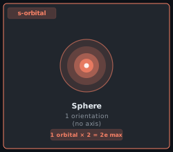
• $\ell =0$ ($s$-subshell): $m_{\ell }$ can only be $0$. (1 orientation, a sphere)
• $\ell =1$ ($p$-subshell): $m_{\ell }$ can be $-1,0,1$. (3 orientations, dumbbells)
• $\ell =2$ ($d$-subshell): $m_{\ell }$ can be $-2,-1,0,1,2$. (5 orientations)
• $\ell =3$ ($f$-subshell): $m_{\ell }$ can be $-3,-2,-1,0,1,2,3$. (7 orientations)

Wait, what about $\ell \ge 4$? 🤔

Mathematically, $\ell$ can be $4,5,6\dots$ ($g,h,i$ subshells). However, none of the 118 known elements in the Periodic Table require these subshells to house their electrons in their ground state. They are mathematically possible but physically unoccupied in the "base model" of our universe.

4.5 The Spherical Harmonics ($Y_{\ell }^{m_{\ell }}$)

When we combine $\mathrm{\Theta }$ and $\mathrm{\Phi }$, we get the Spherical Harmonics:

$$Y_{\ell }^{m_{\ell }}(\theta ,\varphi )\propto P_{\ell }^{m_{\ell }}(\cos \theta )\exp (i{m}_{\ell }\varphi )$$

These functions are the "building blocks" of atomic shapes. By plotting the probability density ($|Y{|}^2$), we reveal the specific geometries of the subshells.

Visualize the solutions? 🤔

Interact with and rotate these exact mathematical shapes: 3D Atomic Orbital Visualizer. For the explicit formulas, see the Mathematical Annex.

• $\ell =0$ ($s$-orbital): Spherically symmetric.
  There are no angular nodes, so the probability of finding the electron is identical in every direction from the nucleus.
• $\ell =1$ ($p$-orbitals): Lobed symmetry.
  Each has a single nodal plane passing through the nucleus, dividing the orbital into two distinct lobes. These align perfectly along the $x,y,$ or $z$ axes ($p_x,p_y,p_z$).
• $\ell =2$ ($d$-orbitals): Quadrant symmetry.
  Most have two perpendicular nodal planes that cross at the nucleus, creating a four-lobed structure. One exception ($d_{z^2}$) has two conical nodal surfaces, resulting in two lobes with a "toroidal" ring around the center.
• $\ell =3$ ($f$-orbitals): Octant symmetry.
  These have three nodal surfaces, resulting in highly complex eight-lobed or multi-ringed geometries.

4.6 Orbital Shapes — Visually

The following diagrams, extracted from the Quantum Principles reference sheet, show the visual form of each orbital type along with its orientation count and capacity.

• s-orbital: Spherical shape, 1 orientation, holds 2 electrons

  

• p-orbitals: Dumbbell shape along 3 axes ($p_x,p_y,p_z$), 3 orientations, holds 6 electrons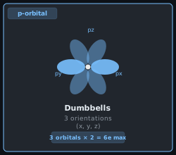

  

• d-orbitals: Four-lobed shapes, 5 orientations, holds 10 electrons

  

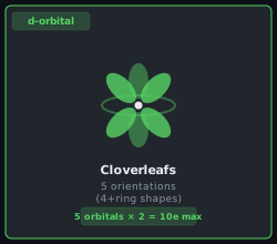
• f-orbitals: Complex multi-lobed shapes, 7 orientations, holds 14 electrons

  

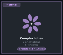
4.7 Summary of the Angular Logic

1. Boundary Condition (Rotation): Requires $m_{\ell }$ to be an integer.
2. Boundary Condition (Finiteness): Requires $\ell$ to be an integer $\ge |m_{\ell }|$.
3. The Result: The geometry of the periodic table blocks ($s,p,d,f$) is a direct physical manifestation of these angular symmetries.

Next, in Chapter 5, we will solve the Radial Equation to find the energy of these shells and finally understand the "Rows" of the table.